How to use Apache Drill

Drill is an Apache open-source SQL query engine for Big Data exploration. Drill is designed  to support high-performance analysis on the semi-structured. It uses ecosystem of ANSI SQL, the industry-standard query language. Drill provides plug-and-play integration with existing Apache Hive and Apache HBase deployments.

Why Drill

Top  Reasons to Use Drill:

1. Get started in minutes:It takes just a few minutes to get started with Drill. 
2. Schema-free JSON model:No need to define and maintain schemas or transform data (ETL). Drill automatically understands the structure of the data.
3. Query complex, semi-structured data in-situ:Using Drill's schema-free JSON model, you can query complex, semi-structured data in situ. No need to flatten or transform the data prior to or during query execution.
4. Leverage standard BI tools:Drill works with standard BI tools. You can use your existing tools, such as Tableau,
5. Access multiple data sources:You can connect Drill out-of-the-box to file systems (local or distributed, such as S3 and HDFS), HBase and Hive
6. High performance:Drill is designed from the ground up for high throughput and low latency. It doesn't use a general purpose execution engine like MapReduce, Tez or Spark. As a result, Drill is flexible (schema-free JSON model) and performant.

High-Level Architecture

At the core of Apache Drill is the "Drillbit" service, which is responsible for accepting requests from the client, processing the queries, and returning results to the client.

A Drillbit service can be installed and run on all of the required nodes in a Hadoop cluster to form a distributed cluster environment. When a Drillbit runs on each data node in the cluster, Drill can maximize data locality during query execution without moving data over the network or between nodes. Drill uses ZooKeeper to maintain cluster membership and health-check information.

Though Drill works in a Hadoop cluster environment, Drill is not tied to Hadoop and can run in any distributed cluster environment. The only pre-requisite for Drill is ZooKeeper.

When you submit a Drill query, a client or an application sends the query in the form of an SQL statement to a Drillbit in the Drill cluster. A Drillbit is the process running on each active Drill node that coordinates, plans, and executes queries, as well as distributes query work across the cluster to maximize data locality.

The following image represents the communication between clients, applications, and Drillbits:

The Drillbit that receives the query from a client or application becomes the Foreman for the query and drives the entire query. A parser in the Foreman parses the SQL, applying custom rules to convert specific SQL operators into a specific logical operator syntax that Drill understands. This collection of logical operators forms a logical plan. The logical plan describes the work required to generate the query results and defines which data sources and operations to apply.

The Foreman sends the logical plan into a cost-based optimizer to optimize the order of SQL operators in a statement and read the logical plan. The optimizer applies various types of rules to rearrange operators and functions into an optimal plan. The optimizer converts the logical plan into a physical plan that describes how to execute the query.

A parallelizer in the Foreman transforms the physical plan into multiple phases, called major and minor fragments. These fragments create a multi-level execution tree that rewrites the query and executes it in parallel against the configured data sources, sending the results back to the client or application.

A major fragment is a concept that represents a phase of the query execution. A phase can consist of one or multiple operations that Drill must perform to execute the query. Drill assigns each major fragment a MajorFragmentID.

For example, to perform a hash aggregation of two files, Drill may create a plan with two major phases (major fragments) where the first phase is dedicated to scanning the two files and the second phase is dedicated to the aggregation of the data.

Drill uses an exchange operator to separate major fragments. 

Major fragments do not actually perform any query tasks. Each major fragment is divided into one or multiple minor fragments (discussed in the next section) that actually execute the operations required to complete the query and return results back to the client.

Each major fragment is parallelized into minor fragments. A minor fragment is a logical unit of work that runs inside a thread. A logical unit of work in Drill is also referred to as a slice. The execution plan that Drill creates is composed of minor fragments. Drill assigns each minor fragment a MinorFragmentID.

The parallelizer in the Foreman creates one or more minor fragments from a major fragment at execution time, by breaking a major fragment into as many minor fragments as it can usefully run at the same time on the cluster.

Drill executes each minor fragment in its own thread as quickly as possible based on its upstream data requirements. Drill schedules the minor fragments on nodes with data locality. Otherwise, Drill schedules them in a round-robin fashion on the existing, available Drillbits.

Minor fragments can run as root, intermediate, or leaf fragments. An execution tree contains only one root fragment. Data flows downstream from the leaf fragments to the root fragment.

The root fragment runs in the Foreman and receives incoming queries, reads metadata from tables, rewrites the queries and routes them to the next level in the serving tree. The other fragments become intermediate or leaf fragments.

Intermediate fragments start work when data is available or fed to them from other fragments. They perform operations on the data and then send the data downstream. They also pass the aggregated results to the root fragment, which performs further aggregation and provides the query results to the client or application.

The leaf fragments scan tables in parallel and communicate with the storage layer or access data on local disk. The leaf fragments pass partial results to the intermediate fragments, which perform parallel operations on intermediate results.

Drill only plans queries that have concurrent running fragments. For example, if 20 available slices exist in the cluster, Drill plans a query that runs no more than 20 minor fragments in a particular major fragment. Drill is optimistic and assumes that it can complete all of the work in parallel. All minor fragments for a particular major fragment start at the same time based on their upstream data dependency.

The following image represents components within each Drillbit:

The following list describes the key components of a Drillbit:

• RPC endpoint: Drill exposes a low overhead protobuf-based RPC protocol to communicate with the clients. 
• SQL parser: Drill uses Calcite, the open source SQL parser framework, to parse incoming queries. The output of the parser component is a language agnostic, computer-friendly logical plan that represents the query.
• Storage plugin interface: Drill serves as a query layer on top of several data sources.In the context of Hadoop, Drill provides storage plugins for distributed files and HBase. Drill also integrates with Hive using a storage plugin.

Drill Session:

You can use a jdbc connection string to connect to SQLLine when Drill is installed in embedded mode or distributed mode, as shown in the following examples:

• Embedded mode:./sqlline -u jdbc:drill:drillbit=local
• Distributed mode:./sqlline –u jdbc:drill:zk=cento23,centos24,centos26:2181

For creating the drill session ,open the putty and type "sqlline".

You can write simple queries of sql like "show databases".It will list all the databases.

Workspaces:
You can create your own workspace in drill. Workspace is nothing but the directory in which you can create your views / tables. You can define one or more workspaces in a storage plugin configuration.

Attribute-workspaces". . . "location

Example-"location": "/Users/johndoe/mydata"

VIEW:

The CREATE VIEW command creates a virtual structure for the result set of a stored query. A view can combine data from multiple underlying data sources and provide the illusion that all of the data is from one source. You can use views to protect sensitive data, for data aggregation, and to hide data complexity from users. You can create Drill views from files in your local and distributed file systems, such as Hive and HBase tables, as well as from existing views or any other available storage plugin data sources.

The CREATE VIEW command supports the following syntax:

CREATE [OR REPLACE] VIEW [workspace.]view_name [ (column_name [, ...]) ] AS query;

Parameters

• workspace:The location where you want the view to exist. By default, the view is created in the current workspace. 
• view_name:The name that you give the view. The view must have a unique name. It cannot have the same name as any other view or table in the workspace.
• column_name:Optional list of column names in the view. If you do not supply column names, they are derived from the query.
• query:A SELECT statement that defines the columns and rows in the view.

The following example shows a writable workspace as defined within the storage plugin in the /DrillView directory of the file system:

"workspaces": {

   "supply_view": {

     "location": "/a/b/DrillView",

     "writable": true,

     "defaultInputFormat": null

   }

 }

Drill stores the view definition in JSON format with the name that you specify when you run the CREATE VIEW command, suffixed by .view.drill. For example, if you create a view named myview, Drill stores the view in the designated workspace as myview.view.drill.

For example, i have created one view dummy in my workspace dfs.supply_view over a hive table employee.

1. Select the workspace by command use dfs.supply_view;
2. Create view dummy as select * from hive.`default`.employee.

Note 1 :You have to use escape character as default is reserved word in drill.

Here you can check your view file in linux file system by going to the workspace directory which you have provided in conf file.

Note 2:For hbase and binary tables you have to use function CONVERT_FROM.

For example

create view dfs.supply_view.mydrill_bang as SELECT CONVERT_FROM(row_key, 'UTF8') AS name, 

CONVERT_FROM(customer.addr.city, 'UTF8') AS city,

CONVERT_FROM(customer.addr.state, 'UTF8') AS state,

CONVERT_FROM(customer.`order`.numb, 'UTF8') AS numb,

CONVERT_FROM(customer.`order`.`date`, 'UTF8') AS `date`

FROM customer

WHERE CONVERT_FROM(customer.addr.city, 'UTF8')='bengaluru';

WEB DRILL

You can run query in Drill web UI  as well.The Drill Web UI is one of several client interfaces that you can use to access Drill

Accessing the Web UI

To access the Drill Web UI, enter the URL appropriate for your Drill configuration. The following list describes the URLs for various Drill configurations:

http://<IP address or host name>:8047
Use this URL when HTTPS support is disabled (the default).
https://<IP address or host name>:8047
Use this URL when HTTPS support is enabled.
http://localhost:8047
Use this URL when running Drill in embedded mode (./drill-embedded).

On accessing drill web UI .It looks like this.

Now click on query ,a window will pop like this.

Now write the query and you will see the results like this.

You can also check the performance of your query by going to the profiles.A profile is a summary of metrics collected for each query that Drill executes. Query profiles provide information that you can use to monitor and analyze query performance. When Drill executes a query, Drill writes the profile of each query to disk, which is either the local filesystem or a distributed file system, such as HDFS.

You can view query profiles in the Profiles tab of the Drill Web UI. When you select the Profiles tab, you see a list of the last 100 queries than ran or are currently running in the cluster.

You must click on a query to see its profile.

The profile hold all the information for the query like physical plan,visualized plan.It conatins all the info like elapsed time between hive ,total fragments,total cost.

By reading all this you can optimise your query and re-write it in a optimised way.

Thats all.

Thanks for reading!

Bye!

Gradient Descent

Hello, and welcome to this blog on  Gradient Descent. 

Derivative:

As the name suggest, a derivative is a function that derives from another function.

Let's start with an example. Imagine you are driving on the highway as time goes by, you mark your position along the highway filling a table of values as a function of time. If you're speed is 60 miles an hour every minute your position will be increased by one mile.

 Let's define the function, x(t) to indicate your position as a function of time. The derivative of this function is the rate of change in position with respect to time.

So the speed will be 

At each point along the curve the derivative is the value of the slope of the curve itself. We can calculate the approximate value of the slope by the method of finite differences. The value of the derivative is negative when the slope of the original curve is downhill and it is positive when the slope is uphill. 

Gradient:

When our function has more than one input we need to specify which variable we are using for derivation. For example, let's say we are measuring our elevation on a mountain as a function of our position. Our GPS position is defined by two variables longitude and latitude. 

elevation=f(long,lati)

And therefore, the elevation depends on two variables. Let's change the variable names to shorter ones. Let's call the elevation y, and the two variables x₁ and x₂

y=f(x1,x2)

We can calculate the rate of change in elevation with respect to x₁, and the rate of change with respect to x₂. 

These are called partial derivatives because we only consider the change with respect to one variable. Notice also that we use the different symbol to indicate these derivatives because these are partial derivatives.

 In the two-dimensional plane of x₁ and x₂, the direction of the most abrupt change will be a two-dimensional vector whose components are the partial derivatives with respect to each variable.

 We call this vector gradient and we indicate it with an inverted triangle 

which is also called del or nabla. 

The gradient is an operation that takes a function of multiple variables and returns a vector. The components of this vector are all the partial derivatives of the function. Since the partial derivatives are functions of all variables, the gradient, too, is a function of all variables.

Back-propagation Intuition:

Let's say we have a function of only one variable called w. For every value on the horizontal axis, the function associates a value on the vertical axis. Let's say we're sitting at a particular point like in the figure.

 Let's also assume that we do not know the function f(w) at every possible point. We only know it near where we are. We want to move in the direction of decreasing f(w), but we can only use local information. How do we decide where to go? As we've when we talked about descending from a hill, the derivative indicates its slope at each point, so we can calculate the derivative where we are, and then change our position by subtracting the value of the derivative from the value of our starting position w. In other words, we can take one step, following the rule 

If we are sitting at w, the slope of the curve is negative, and thus, the quantity minus

 is positive, so the value of w will increase.So we have to move towards the right on the horizontal axis.  So the corresponding value on the vertical axis will decrease, so we successfully moved towards the lower value of the function f of w. 

This way of looking for the minimum of a function is called gradient descent, and it's the idea behind back-propagation. Given a function, we can always move towards its minimum by following the path indicated by its derivative, or, in the case of multiple variables, indicated by the gradient. As you know by now, for a neural network, we define a cost function that depends on the values of the parameters, and as you also know, we find the values of the parameters by minimizing the cost by gradient descent. All we are really doing is taking the cost function, calculating its partial derivatives with respect to each parameter, and then using the update rule we just described to decrease the cost by updating the parameter. We do this by subtracting the value of the negative gradient from each of the parameters. 

This is what's called a parameter update.

 Learning Rate:

As noted, the gradient vector has both a direction and a magnitude. Gradient descent algorithms multiply the gradient by a scalar known as the learning rate (also sometimes called step size) to determine the next point. For example, if the gradient magnitude is 2.5 and the learning rate is 0.01, then the gradient descent algorithm will pick the next point 0.025 away from the previous point.

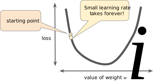
Hyperparameters are the knobs that programmers tweak in machine learning algorithms. Most machine learning programmers spend a fair amount of time tuning the learning rate. If you pick a learning rate that is too small, learning will take too long:

Learning rate is too small.

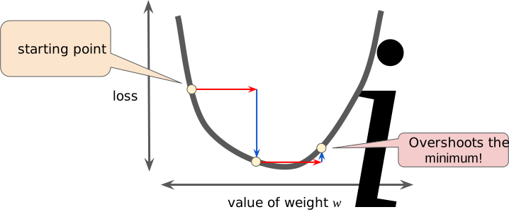
Conversely, if you specify a learning rate that is too large, the next point will perpetually bounce haphazardly across the bottom of the well like a quantum mechanics experiment gone horribly wrong:

Learning rate is too large.

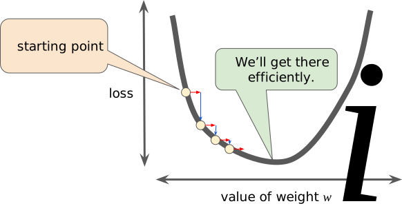
There's a Goldilocks learning rate for every regression problem. The Goldilocks value is related to how flat the loss function is. If you know the gradient of the loss function is small then you can safely try a larger learning rate, which compensates for the small gradient and results in a larger step size.

Learning rate is just right.

Reducing Loss: Stochastic Gradient Descent

In gradient descent, a batch is the total number of examples you use to calculate the gradient in a single iteration. So far, we've assumed that the batch has been the entire data set. But in real time the data sets often contain billions or even hundreds of billions of examples. Consequently, a batch can be enormous. A very large batch may cause even a single iteration to take a very long time to compute.

A large data set with randomly sampled examples probably contains redundant data. In fact, redundancy becomes more likely as the batch size grows. Some redundancy can be useful to smooth out noisy gradients, but enormous batches tend not to carry much more predictive value than large batches.

What if we could get the right gradient on average for much less computation? By choosing examples at random from our data set, we could estimate (albeit, noisily) a big average from a much smaller one. Stochastic gradient descent (SGD) takes this idea to the extreme--it uses only a single example (a batch size of 1) per iteration. Given enough iterations, SGD works but is very noisy. The term "stochastic" indicates that the one example comprising each batch is chosen at random.

Mini-batch stochastic gradient descent (mini-batch SGD) is a compromise between full-batch iteration and SGD. A mini-batch is typically between 10 and 1,000 examples, chosen at random. Mini-batch SGD reduces the amount of noise in SGD but is still more efficient than full-batch.

Introduction of Machine Learning

Today,I am writing on machine learning..everybody is speaking about this machine learning but what is machine learning? Do we really know that..

Machine learning involves building mathematical models to help understand data. 

“Learning” comes into picture when we give these models tunable parameters that can be adapted to observed data; in this way the program can be considered to be “learning” from the data. Once these models have been fit to previously seen data, they can be used to predict and understand aspects of newly observed data.

Machine learning is the process where we actually moving our logic into statistics. 

Some Important terminologies:

1)Label:

A label is the thing we are predicting.The 'y' variable in the linear regression is the label.It can be anything like price of house,kind of bird shown in picture etc.

2)Feature:

Feature is the input variable.'x' in the linear regression is feature. A simple machine learning project might use a single feature, while a more sophisticated machine learning project could use millions of features, specified as:

X_1,X2,X3......Xn

Types of Learning:

1) Supervised Learning:

Supervised learning is where when you have feature and label and you use an algorithm to learn the mapping function from the input to the output.

Y = f(X)

The goal is to approximate the mapping function so well that when you have new feature (input data (x)) that you can predict the label (output variables (Y)) for that data.

It is called supervised learning because the process of an algorithm learning from the training dataset can be thought of as a teacher supervising the learning process. We know the correct answers, the algorithm iteratively makes predictions on the training data and is corrected by the teacher. Learning stops when the algorithm achieves an acceptable level of performance

Supervised learning problems can be further grouped into regression and classification problems:

Regression vs. classification

A regression model predicts continuous values. For example, regression models make predictions that answer questions like the following:

What is the value of a house in California?

What is the probability that a user will click on this ad?

A classification model predicts discrete values. For example, classification models make predictions that answer questions like the following:

Is a given email message spam or not spam?

Is this an image of a dog, a cat, or a hamster?

2)Unsupervised Learning:

Unsupervised learning is where you only have feature (input data (X)) and no corresponding label (output variables (Y)).

The goal for unsupervised learning is to model the underlying structure or distribution in the data in order to learn more about the data.

These are called unsupervised learning because unlike supervised learning above there is no correct answers and there is no teacher. Algorithms are left to their own devises to discover and present the interesting structure in the data

3)Semi-supervised Learning:

Problems where you have a large amount of input data (X) and only some of the data is labeled (Y) are called semi-supervised learning problems.

These problems sit in between both supervised and unsupervised learning.

A good example is a photo archive where only some of the images are labeled, (e.g. dog, cat, person) and the majority are unlabeled.

Wherescape Red Tool

Traditionally data warehouses take too long to build and are too hard to change. WhereScape RED is an Integrated Development Environment to support the building and managing of data warehouses.
It has the flexibility to enable you to build a variety of architectures including:

• enterprise data warehouses
• dimensional data warehouses
• data marts
• user facing views, aggregates and summaries

In all cases the core values of WhereScape RED are twofold: its rapid building capabilities that enable better data warehouses to be built, faster, and its integrated environment that simplifies management.

As a data warehouse specific tool, WhereScape RED embodies a simple, pragmatic approach to building data warehouses. With WhereScape RED you specify what you want to achieve by dragging and dropping objects to create a meta view, and then let WhereScape RED do the heavy lifting of creating the necessary tables and procedures etc. Data warehouse wizards prompt for additional information at critical points to provide the maximum value from the generated objects.

WhereScape RED supports these concepts to facilitate very rapid delivery of data warehouses. WhereScape RED controls the flow of data from the source systems through transforming and modeling layers to analysis areas.

Different styles of data warehousing (EDW 3NF, dimensional etc) are supported and utilize different objects, but all follow the same basic flow.

1. Data Flow - Enterprise Models
2. Source (OLTP) System
3. load tables
4. stage tables
5. data store tables
6. model tables, dimension tables, or detailed (transactional) fact tables
7. roll up fact table(s)
8. aggregate and/or KPI fact table(s)
9. views
10. export objects
11. Microsoft Analysis Services cubes

The diagram below shows the objects and the information flow:

Data Flow:

Data is moved from source tables to load tables via scripts, database links and ODBC links. These load tables are created by dragging and dropping from a connection object. Load tables are generally based on source system tables. Their main purpose is to be a destination for moving data as simply and quickly as possible from the source system. Load tables will generally hold a single unit of data (e.g. last night or last month), and will be truncated at the start of each extract. Transformations can be performed on the columns during the load process if required.

Load tables feed stage tables, which in turn feed data store, model or dimension tables. Data from multiple load tables can be combined at this level.

First tier transactional tables (fact or model) are created and updated from stage tables. Second tier tables (model, summary rollup, aggregate, KPI, etc.) are created and updated from lower level tables.

Cubes can be created from transactional tables or views.

Procedural code:

WhereScape RED generates procedural code in the target database's native language (e.g. PL/SQL for Oracle) at each stage in the data warehouse build process. The generated code is, in nearly all cases, sufficient to create a rapid prototype of the data warehouse.

While the generation of code is often seen as a key benefit of WhereScape RED, the ability to control and manage custom code is also critical to the long term management of the data warehouse environment.

In most cases 85-100% of the generated code will be taken through to production with no customization required.

WhereScape RED and Traditional ETL Tools:

WhereScape RED's core strength is in the rapid building of data warehouse structures. Organizations that have already purchased traditional ETL tools can use WhereScape RED as a pureplay data warehouse toolset. WhereScape RED can be used to iteratively build data marts or presentation layer objects that need to be constantly updated to keep relevant for end users. In most cases, customers will find that WhereScape RED has enough ETL capabilities to build the entire data warehouse, using the database rather than a proprietary engine to perform ETL processing.

The cross over in functionality between ETL tools and WhereScape RED is not large. WhereScape RED is tightly integrated into the data warehouse database and has an embedded data warehouse building approach. For WhereScape data movement is the start of the process—from source system to load tables. The key benefits of the product: development productivity and an integrated environment to manage and maintain your data warehouse, comes after the data movement stage. Where a traditional ETL tool is already in use, the output of the ETL process is a WhereScape RED Load, Stage, Dimension, Fact or Model table from which WhereScape RED builds more advanced data warehouse structures.

Data Vault: 

The Data Vault system is an alternative approach to modelling an enterprise data warehouse that has been gaining popularity among organizations.

The Data Vault data warehouse architecture was invented by Dan Linstedt to provide an alternative to the traditional data warehouse modelling approach that includes developing 3rd Normal Form (3NF) type models or dimensional star schema models. The data vault methodology seeks to improve the efficiency of data ingestion and the flexibility of structure changes. 

WhereScape RED has been enhanced to expand its current Data Vault functionality and provide improved automation for creating and managing Data Vault objects in WhereScape RED managed Data Warehouses. The enhancement includes the following:

1. New DSS columns for Load tables
2. New Wizard for Hash key generation
3. New Wizard for building Hub, Link and Satellite tables
4. New Templates for Procedure generation

The Hub, Link and Satellite tables are based on standard Load or Stage tables (that do not include the hash key column type flags) then WhereScape RED reverts to this behavior and the resulting procedures are generated by internal WhereScape RED automation and not via templates.

Here I am describing how to load data from the SAP Hana system to Hadoop environment using by wherescape RED Tool.

This comprises four types of Data loads for each individual table stream. Initial step would be Loading in a straight line from the Hana System, before we are moving it to Hadoop make sure to create the Source connection with HANA and to be established. Following connection made to be available with attached connection information

Hadoop Cluster Connection:

This connection is basically to get connected to Hadoop clusters to create and Load/verify the tables and before loading into Hadoop table, we have verified the schema which has created correctly or not. Basically, Data would be loaded into hadoop table in various formats depends on our requirements. 

Now we load the data by the sqoop scripts.

 

Steps to be performed:

Step:1

Select the table from source DB which we are loading into Hadoop cluster, primarily all the data will be pushed to hive external tables.(we are moving into hive tables just now for storage )
Drag the table and create it as Load table
Once the we create the table, select the properties and choose the following connectivity to create the script.

·         Connection details for source
·         Load type based on the scripts
·         Connection type should be always Linux
·         Select the Sqoop script template
·         Choose the template sqoop

We can see it from the below snapshot for detailed information

 

 By clicking the generate tab, it will create the scope script along with source table columns and description Once we have generated the code kindly create the table by using a hive DDL template as to defy in drop-down list. Make sure to check the table creation in hive Metastore then start the Load to consume the data from Hana

 

                                                                                                     

Once we done the property's activity, please click on generate scripts in the properties tab. Postscript generation please verify the script for confirmation. Right click on table execute load function. Once the load completes, start the Stage table

 

Step:2

Now we move the table into stage layer.

Stage tables are used to transform the data to a star schema or third normal form model. A stage table can be a fact or an EDW. 3NF table that only contains change data or a work table. In star schema data warehouses, the stage table brings all the dimensional joins together in preparation for publishing into the fact table.

A stage table is built from the Data Warehouse connection. Unless you are retrofitting an existing system, stage tables are typically built from one or more load or stage tables. They can utilize the surrogate keys from a number of dimension tables.

The use of this table is loading is to create the Hub Key and change key to make no data is missing when it moved to further steps Before running the update script, please verify the table in source Before generating the Key Column to bring the key from the source table.

                                                                                                     

 

• Click Rebuild Option to select the template options.

• Once the template is selected, click on properties Regenerate. This should prompt to select HubKey and Changekey. Hub Key should hold the hash of primary key and changekey should hold hash of remaining keys concatenated together. Click on “OK”.
• Once we done the property's activity, please click on generate scripts in the properties tab. Postscript generation please verify the script for confirmation. Right click on table execute “Run Update script” function. Once the load completes, start the Hub table Loading.

Fact Table:

A Fact table is normally defined, for our purposes, as a table with facts (measures) and dimensional keys that allow the linking of multiple dimensions. It is normally illustrated in the form of a Star Schema with the central Fact table and the outlying dimensions.

The ultimate goal of the Fact table is to provide business information to the end user community. In many cases, different types of Fact tables are required to address different end user requirements. For simplicity, the different types of fact table are grouped together under the following headings:

Hub Table:

Hubs contain a list of unique business keys with low propensity to change. Hubs also contain a surrogate key for each Hub item and metadata describing the origin of the business key. The descriptive attributes for the information on the Hub (such as the description for the key, possibly in multiple languages) are stored in structures called Satellite tables which will be discussed below.

Links:

Associations or transactions between business keys (relating for instance the hubs for customer and product with each other through the purchase transaction) are modeled using link tables. These tables are basically many-to-many join tables, with some metadata.

Links can link to other links, to deal with changes in granularity (for instance, adding a new key to a database table would change the grain of the database table). 

Satellites:

The hubs and links form the structure of the model, but have no temporal attributes and hold no descriptive attributes. These are stored in separate tables called satellites. These consist of metadata linking them to their parent hub or link, metadata describing the origin of the association and attributes, as well as a timeline with start and end dates for the attribute. Where the hubs and links provide the structure of the model, the satellites provide the "meat" of the model, the context for the business processes that are captured in hubs and links. 

Step:3

Hub Table:

This table holds Business keys and generated hub keys. Create a Hub table utilizing the above created Stage table (either by creating new hub table and then mapping with stage columns or by dragging the source table in to Column View pane).

1.  In the Table Column view Pane, select Primary Business Key and the Hash Key.
2.  Create MaprDB table manually in the required MAPR path.
3.  Right click on the Newly Created Hub Table and select “Properties”
4. Use Storage and Extended properties as show in the above figure to select DDL template (make sure to select appropriate MARDB table location in MARDB location.
5. Click on Rebuild to select required template and once the template is selected, click on “Regenerate” to generate the script.
6.  Postscript generation please verify the script for confirmation. Right click on table and click “Create(Recreate)” option to create “HIVE_MAPRDB” interface table.
7.  Once the table got created, right click on the table, and select “Execute Update script” to load the data into HIVE_MAPRDB interface table.

Step:4

Satellite table:

Satellites have metadata linking them to their parent hub , metadata describing the origin of the association and attributes, as well as a timeline with start and end dates for the attribute. Where the hubs and links provide the structure of the model, the satellites provide the "meat" of the model, the context for the business processes that are captured in hubs and links.

1. Create a Satellite table utilizing the above created Stage table (either by creating new hub table and then mapping with stage columns or by dragging the source table in to Column View pane).
2. In the Table Column view Pane, select Hash Key and the change key .
3.  Add a new column which holds “updated_date” i.e the time when record got inserted. This along with Change key will act as unique key for satellite table.
4. Create Maprfs table in the required maprfs path.
5. Right click on the Newly Created Hub Table and select “Properties”
6. Use Storage and Extended properties as show in the above figure to select DDL template (make sure to select appropriate MARDB table location in MARDB location.
7. Click on Rebuild to select required template and once the template is selected, click on “Regenerate” to generate the script.
8. Postscript generation please verify the script for confirmation. Right click on table and click “Create(Recreate)” option to create “HIVE_MAPRDB” interface table.
9. Once the table got created, right click on the table, and select “Execute Update script” to load the data into HIVE_MAPRDB interface table.

Here is the end of blog.

Thanks for reading..Bye.